Online self-study course 1: Introduction to R using a protocol for conducting and presenting results of regression-type analyses.

Course format:

• Self-study course.
• On-demand access to all video content online within a 12-month period.
• Daily interaction on the Discussion Board for detailed questions.
• Live chat for quick queries.
• Course fee includes a 1-hour video chat with instructors for personalized questions and data assistance.

Course content

In this course, we will provide an introduction to R and simultaneously explain how to conduct data exploration, apply (simple) linear regression models, communicate results, and determine the optimal sample size (using power analysis) in case you intend to set up a new field study or experiment.

We will follow a 10-step protocol based on Zuur and Ieno (2016). This protocol will guide us through the process of organizing data (including formulating relevant questions, visualizing data collection, performing dat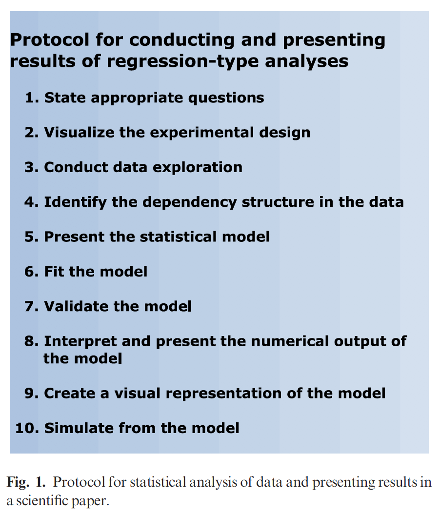a exploration, and identifying dependencies), conducting analysis (presenting, fitting, and validating the model), and presenting output (both numerically and visually), eventually extending the model through simulation.

This course is designed for scientists who want to learn R through a non-traditional approach, applying it in a playful manner. It's also beneficial for scientists who have completed an introductory R course and wish to advance their skills to the next level. The course covers topics such as data exploration, data visualization, the application of linear regression models, and power analysis.

The online course is divided into various modules, amounting to approximately 10 hours of work in total. Each module comprises multiple video files featuring brief theoretical presentations, followed by exercises using real datasets, and video discussions of the solutions.

Module 1

We begin this module with a theory presentation based on Zuur and Ieno (2015. Following a 10-step protocol, we will explain how to conduct a regression-type analysis and present the results. Please note that we won't delve too deeply into the statistical theory that underlies the models.

Next, we'll engage in three exercises designed to teach you how to import data, manipulate data (including actions like deleting rows and selecting columns), create data visualizations using ggplot2, and formulate questions to prepare for statistical analysis.

A more detailed outline is provided through the following two bullet points:

• Introduction to R, including a theory presentation on the 10-step protocol and the execution of steps 1 and 2 of the protocol using R. This segment will encompass discussions about installing R, R-Studio, add-on packages, importing data into R, and accessing variables.
• Presentation of various datasets, accompanied by a discussion on how to formulate the underlying questions (which will drive the application of specific statistical techniques). We will leverage the ggplot package in R to visualize spatial-temporal data and explain how to modify and manipulate datasets in R (such as removing rows or columns, and creating new variables).

Module 2

In this module, we kick off with a theoretical presentation on data exploration, drawing from Zuur et al. (2010). We will put data exploration into practice using three datasets. We'll cover the identification and management of outliers, and delve into methods to recognize collinearity (correlation between covariates). Techniques including multipanel scatterplots, Pearson correlations, variance inflation factors, and principal component analysis biplots will be explained in straightforward terms. It's essential to note that we will also debunk the misconception of testing response variables for normality.

The following bullet points summarize module 2:

• Carrying out data exploration in R and visualizing the data's dependency structure (comprising steps 3 and 4 of the protocol).
• Continuing with the visualization of spatial data, time-series data, and spatial-temporal data. This exploration will involve utilizing R functions like plot, boxplot, and dotchart. We'll emphasize the ggplot2 package to craft multipanel graphs.

Module 3

The third module encompasses three exercises. In the first exercise, we will execute a linear regression model with one covariate and apply the complete protocol. We'll guide you through model application, interpreting output, assessing model goodness through validation, and visualizing outcomes using ggplot2. The second exercise involves a linear regression model with two covariates, where we'll follow the same protocol. While we'll use a simple linear regression model, the same steps can be extended to more advanced models like linear mixed-effects models, GLMMs, or GAM(M)s.

For the third exercise, we'll revisit one of the datasets used earlier in the course. The question we'll address is: "If we were to repeat the sampling process, how many observations should we take?" This query will be addressed through 'power analysis,' a statistical tool surprisingly simple in its application. We'll employ power analysis to explore the implications of taking fewer or more observations. Additionally, we'll investigate the number of observations required to detect a 20% change, a 10% change, and a 5% change in the response variable. The efficiency of power analysis in terms of cost and time will be highlighted. We'll even guide you through programming power analysis from scratch. It's worth noting that power analysis can also be extended to more advanced models like GLMM (though this falls outside the scope of this course).

The following bullet points encapsulate the content of the third module:

• Two exercises implementing steps 5 to 10 of the protocol.
• We'll assume you have a basic understanding of linear regression (providing a layman's explanation). We'll demonstrate how to implement such a model in R, clarify how to evaluate underlying assumptions, and showcase visualization techniques.
• Detailed guidance on presenting findings in a paper or report.
• One exercise dedicated to explaining and applying power analysis to ascertain optimal sample size.

Prerequisite Knowledge

Basic statistics (such as mean, variance, normality) are assumed prerequisites. No prior knowledge of R is required; you'll pick up R skills as you progress. This is a non-technical course designed for accessibility.